Power BI month-over-month change and a 3-month moving average in DAX
“Are we up or down versus last year?” is the first question a sales report has to answer. The second question — “are we still growing, or has the trend turned?” — is harder, because a single month is noisy: a short month, a late invoice, or one big order can move it by a fifth. This guide builds the short-term view properly: a calendar table, a relationship, and four measures. The headline result: October 2025 revenue of $13,436.42 against $13,415.30 in September 2025, up 0.16% month over month, and the 3-month moving average reached $13,377.24, the highest value in the data.
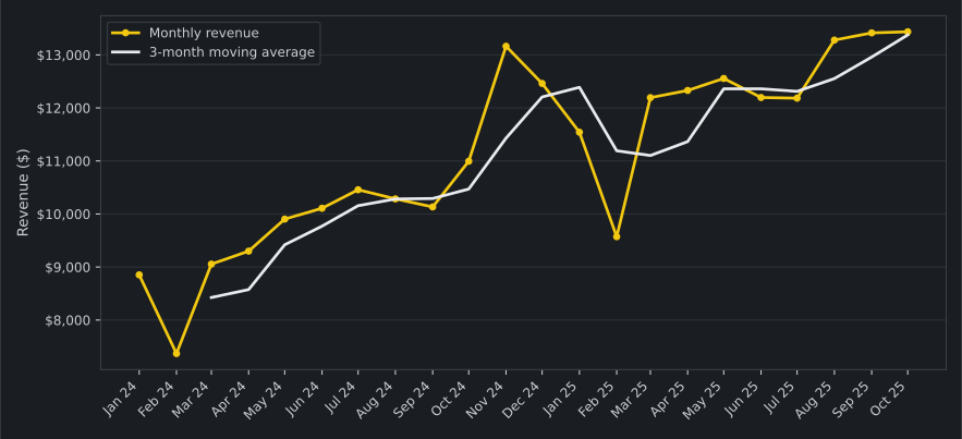
Key result: In October 2025, revenue was $13,436.42, against $13,415.30 in September 2025 — MoM +0.16%. The 3-month moving average was $13,377.24 (August $13,279.99, September $13,415.30, October $13,436.42). January–October 2025 totals $122,707.17.
Download the data and the measures: the sales file (CSV) (66 rows, MD5 51a16fd9e023dd0208564a0c2c1a089e) and the measures file (DAX) (the four measures below, ready to paste). The data is a constructed sample — three product lines, monthly revenue from January 2024 to October 2025 — not a real company's sales.
What you need
- Power BI Desktop on Windows. Desktop is a Windows application; there is no macOS or Linux version, and no headless runner.
- The sample file the sales file (CSV): columns
Month,Category,Units, andRevenue. One row per category per month, 66 rows. - Nothing else. No database, no service, no account.
1. Import the sales file
In Power BI Desktop, go to Home > Get data > Text/CSV, pick the sales file, and choose Load. Check the column types after loading: Month must be a date, Revenue a decimal number, and Units a whole number. If Month loads as text, the relationship in step 3 will not work — change the type in Power Query first.
2. Build the calendar table
Time-intelligence functions need a date table: a table with one row per day, continuous, with no gaps. Microsoft's documentation says to mark one of the tables containing a date column as the date table before using time-intelligence functions (Microsoft Learn — Set and use date tables in Power BI Desktop). Create it as a calculated table:
Calendar =
ADDCOLUMNS (
    CALENDAR ( DATE ( 2024, 1, 1 ), DATE ( 2025, 12, 31 ) ),
    "Year", YEAR ( [Date] ),
    "MonthNumber", MONTH ( [Date] ),
    "MonthName", FORMAT ( [Date], "mmmm" ),
    "Quarter", "Q" & FORMAT ( [Date], "Q" ),
    "MonthYear", FORMAT ( [Date], "mmm yyyy" )
)
CALENDAR on its own returns a table with a single Date column. ADDCOLUMNS adds the columns the visuals need: Year and MonthNumber as numbers, MonthName as the full month name, Quarter as Q1 to Q4, and MonthYear as a label such as Jan 2025. Marking the table as the date table removes the built-in date hierarchies Desktop would otherwise generate. Build one by hand instead: in the Fields pane, right-click Year and choose Add to hierarchy > New hierarchy. Then drag Quarter and MonthName in below Year, in that order. Then sort the months in calendar order: select MonthName and choose Sort by column > MonthNumber on the Column tools ribbon. The full treatment is in Build a Power BI date table in DAX.
Then mark it: select the Calendar table in the Fields pane, right-click, and choose Mark as date table > Mark as date table, with Date as the date column. The same Learn page describes both the right-click path and the Table tools ribbon path. The range must cover every month in the sales file — January 2024 through October 2025 — or the prior-month lookup in step 4 returns blank for the uncovered months.
3. Relate the two tables
In Model view, drag Calendar[Date] onto Sales[Month]. The relationship is one-to-many, single direction, from Calendar to Sales. One calendar date matches many sales rows; no sales row matches more than one calendar date. If the relationship shows as many-to-many or inactive, the Month column is the wrong type — go back to step 1 and fix it.
4. Write the four measures
Create each measure on the Sales table (Modeling > New measure). The measures file (DAX) holds the same four measures, ready to paste.
Total Sales = SUM ( Sales[Revenue] )

Sales PM =
CALCULATE (
    [Total Sales],
    PREVIOUSMONTH ( Calendar[Date] )
)

MoM % Change =
DIVIDE (
    [Total Sales] - [Sales PM],
    [Sales PM]
)

3-Month Moving Average =
AVERAGEX (
    DATESINPERIOD (
        Calendar[Date],
        MAX ( Calendar[Date] ),
        -3,
        MONTH
    ),
    [Total Sales]
)
How it works: PREVIOUSMONTH returns all the dates from the previous month, based on the first date in the current context — Microsoft's own example builds a previous-month sales measure the same way, with CALCULATE and PREVIOUSMONTH (Microsoft Learn, PREVIOUSMONTH function (DAX)). DATESINPERIOD returns a table of dates that begins at a start date and continues for the specified number of intervals; a negative interval shifts backward, and Microsoft's example uses MAX to take the latest date in the filter context as the start (Microsoft Learn, DATESINPERIOD function (DAX)). With MAX ( Calendar[Date] ) as the last day of the current month and -3, MONTH, the window is the current month plus the two before it — for October 2025, 1 August to 31 October. AVERAGEX evaluates an expression for each row of a table and takes the arithmetic mean, following the same rules as AVERAGE (Microsoft Learn, AVERAGEX function (DAX)). CALCULATE reevaluates [Total Sales] under the shifted context, which is how the prior-month figure appears (Microsoft Learn, CALCULATE function (DAX)). DIVIDE handles the empty prior month: a month with no sales the month before returns blank instead of an error (Microsoft Learn, DIVIDE function (DAX)).
One detail matters for the moving average. AVERAGEX iterates over the days in the window, and [Total Sales] is evaluated for each day. The sales file records revenue on the first of each month only, so only three days in any window carry a value, and the blank days are skipped, as AVERAGEX follows the rules of AVERAGE. The result is the average of the three monthly totals. See the second trap below if your own data is daily.
5. Put them in a visual
Add a line chart. Put the Calendar hierarchy (Year > Quarter > MonthName) on the x-axis and drill to the month level. Use [Total Sales] and [3-Month Moving Average] as the values, and add a card visual showing [MoM % Change] formatted as a percentage with two decimals. The moving-average line is the trend; the monthly line is the noise around it. When the monthly line crosses above its moving average after sitting below it, the trend has turned up — in this data that happens in March 2025, after February's drop.
6. Check the numbers
Put the Calendar hierarchy (Year > Quarter > MonthName), drilled to the month level, [Total Sales], [Sales PM], [MoM % Change], and [3-Month Moving Average] in a table visual. Every row must match this table, which was computed independently from the same CSV:
| Month | Total Sales ($) | Sales PM ($) | MoM % | 3-Mo Moving Avg ($) |
|---|---|---|---|---|
| January 2025 | 11,542.57 | 12,461.76 | -7.38% | 12,389.26 |
| February 2025 | 9,571.47 | 11,542.57 | -17.08% | 11,191.93 |
| March 2025 | 12,194.25 | 9,571.47 | +27.40% | 11,102.76 |
| April 2025 | 12,329.83 | 12,194.25 | +1.11% | 11,365.18 |
| May 2025 | 12,556.42 | 12,329.83 | +1.84% | 12,360.17 |
| June 2025 | 12,196.70 | 12,556.42 | -2.86% | 12,360.98 |
| July 2025 | 12,184.22 | 12,196.70 | -0.10% | 12,312.45 |
| August 2025 | 13,279.99 | 12,184.22 | +8.99% | 12,553.64 |
| September 2025 | 13,415.30 | 13,279.99 | +1.02% | 12,959.84 |
| October 2025 | 13,436.42 | 13,415.30 | +0.16% | 13,377.24 |
| Jan–Oct 2025 | 122,707.17 | — | — | — |
If a month shows a blank Sales PM, the calendar table is the suspect: either it was not marked as the date table, or its range does not cover the prior month. If every Sales PM equals Total Sales, the relationship is not filtering the calendar — check step 3. If the moving average equals Total Sales in every row, the DATESINPERIOD window is not reaching back: check that MAX ( Calendar[Date] ) is inside the DATESINPERIOD call, not outside it.
Traps
TRAP — NO DATE TABLE, NO PRIOR MONTH. PREVIOUSMONTH against the sales table's own Month column returns blank, not an error, because the function shifts dates that exist in the date column — and a month-level column has no daily context to shift. The visual looks fine and the numbers are empty. Build and mark the calendar table first.
TRAP — THE MOVING AVERAGE AVERAGES DAYS, NOT MONTHS. AVERAGEX over a DATESINPERIOD window iterates over days, so with daily sales data this measure returns the average daily sales over the window, not the average monthly sales. It returns the average of three monthly totals here only because the sales file has one revenue row per month. With daily data, average the monthly totals instead: iterate over the months with VALUES on a month column, or divide a three-month total by three.
TRAP — A PARTIAL CURRENT MONTH. The month-over-month change compares the current month against a full month. If the file is updated mid-month, the current month is partial and the change reads as a collapse that is not real. Either wait for the month to close or compare only completed months; the moving average has the same problem, since a partial month drags it down for three months running.
End state
A calendar table marked as the date table, a one-to-many relationship to sales, and four measures. The table visual shows ten months of 2025 against the month before each: the change ranged from -17.08% in February to +27.40% in March, and the 3-month moving average bottomed at $11,102.76 in March, then climbed to $13,377.24 by October, dipping only in July. October itself was nearly flat month over month (+0.16%), but the moving average says the trend is still up. The same four measures work on any sales table with a date column and a calendar table — only the table and column names change.
Sources
- Microsoft Learn, PREVIOUSMONTH function (DAX) — returns all dates from the previous month, based on the first date in the current context; the page's example builds a previous-month sales measure with CALCULATE
- Microsoft Learn, DATESINPERIOD function (DAX) — returns dates beginning at a start date and continuing for a number of intervals; a negative interval shifts backward; the page's example uses MAX for the latest date in context
- Microsoft Learn, AVERAGEX function (DAX) — evaluates an expression for each row of a table and takes the arithmetic mean; follows the same rules as AVERAGE
- Microsoft Learn, DIVIDE function (DAX) — returns BLANK on division by zero when no alternate result is given
- Microsoft Learn, CALCULATE function (DAX) — evaluates an expression in a modified filter context
- Microsoft Learn — Set and use date tables in Power BI Desktop — when a date table must be marked, and how to mark it
Checked 11 November 2026. The measure results in the check table were computed in Python 3.12.3 with pandas 2.1.4 by grouping the same sales file by month, shifting one month back, and averaging each month with the two before it — the identical aggregations the DAX performs. October 2025: $13,436.42 vs $13,415.30 in September 2025, +0.16%; 3-month moving average $13,377.24. January–October 2025: $122,707.17. Run the check table against your own report; if a row disagrees, the model differs from the one described above.